Fiat Money Begins: A mathematically based theory of money creation and destruction.
Abstract
An independent theory of fiat money creation based on a mathematical foundation. Modern Money Theory (MMT) advocates will find many parallels but also differences, particularly in the role of banks as creators of money. When the Federal Reserve works with the Federal Treasury to create money, "double money" is created, providing a path to control value. The resulting theory is a logical and coherent explanation of money, money supply and the economy as measured by GDP. The simple formulas used should not be a barrier for beginning students.
Fiat Money Begins
by Roger Sparks
Modern fiat money begins when Government wants to accomplish a goal or apply Keynesian Stimulation. Government issues a promise in exchange for citizens going to work producing goods and services. A promise by Government can be seen as money, debt, evidence-of-debt or a gift certificate. In theory, this promise by Government is without cost to government because, as the citizens exchange the promise for goods, Government recovers the promise a little at a time when taxes are paid at each exchange. Excepting a negligibly small remainder, after a large number of exchanges, all the promises (money) are fulfilled and disappear when tax returns all the money to Government hands, and then the process must begin again. Notice that this process intentionally moves citizens from an assumed stable situation into a dynamic situation with action(s) occurring, a condition of temporary instability.
One major problem made observable by this theory is that, while the initial issue is upfront,money only returns to Government after MANY exchanges, much to the frustration of Government planners. Many people (savers) delay spending the money by saving for a rainy day, a new house, old age, or simply receive in one measurement period and spend in a second, thus delaying the return of money to Government. Naturally, those who delay spending expect to have the same value of exchange in later years as may exist at time of receipt of the money. They want a long term stable money promise, a desire which is directly opposed to the short term efforts of Keynesian stimulators.
At this point, the initial upfront Keynesian action can be seen to have accomplished the original something. Government has recovered some money through taxes and Government finds that some money is held in the hands of savers. The economy now slows because of a money supply shortage, awaiting the spending decisions of savers.
Governments who want people working will, at this point, be tempted to again apply Keynesian Stimulus. If they do this, the above cycle repeats with additional destabilizing effect. More money is added to the economy which then competes with the money already present. History is filled with examples of inflation which is simply the dilution of the value of money.
Use Math to Describe Creation of the Money Supply
The effect of any initial issue of money on Gross Domestic Product (GDP) can be described by
(1) GDP = EMS/ETR
where ETR is the Effective Tax Rate and EMS is the Effective Money Supply. Here, GDP is the upper limit of the sum of all transactions using the original money supply with each successive transaction smaller by the tax withdrawn. Equation 1 is found by describing the shrinking remainder as a Taylor series and solving to find the series limit, which would be GDP.
In a real and stable world, daily money flow is maintained with continuous reissue of existing money. Money is spent by government as fast as it is returned by taxes. If the withdrawal of the money supply equals the insertion rate (a balanced budget), the effective tax on the money supply is zero.
Government records money spent and received. The equation
(2) T + PB = G
describes the accounting identity that Taxes (T) added to Printed or Borrowed (PB) money equals Government (G) expenses. When taxes equal expenses, PB is zero and the money supply is replaced as fast as it is extracted from the economy. When PB is not zero, money is either added to or removed from the money supply. Figure 1 depicts how this government accounting identity is related to GDP.
The government accounting identity (Equation 2) can be arithmetically linked to GDP by dividing both sides of the equation by GDP to get
(3) T/GDP + PB/GDP = G/GDP.
The first term in Equation 3 is the tax rate (TR) and the second term is the Printed/Borrowed Rate (PBR). We can substitute these two terms into Equation 3 and rearrange to get
(4) GDP = G/(TR + PBR)
which will be useful later when we discuss the velocity of money.
Looking at Equation 4, if G is government expenses and considered to be the annual money supply, and PBR is zero for a balanced government budget, equation 4 becomes very similar to Equation 1. This similarity will be developed further in this paper by assuming that the expenses of government are the effective money supply for a fiat money economy.
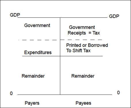
Figure 1: A depiction of the makeup of GDP. GDP includes metrics of Government and a Remainder that is about four times larger than the Government components.
Role of Government in Money Creation
It is worthwhile to reemphasize the unique role of government at the beginning of fiat money in a different context. Only government is allowed to print money. Producers of counterfeit money are quickly dealt with and counterfeit money is removed and destroyed. Any receiver of counterfeit currency finds himself with confiscated or valueless money. The source is the difference between having paper with value or paper with no value.
Because source is only difference between valued money and counterfeit money, careful records must be kept of how much correctly sourced money has been printed and issued. In the United States, beginning in 1913 with the creation of the Federal Reserve, all money has been printed by the Federal Reserve and given to the Government in exchange for Government Debt, OR,the new money has been borrowed from citizens who act identical to the Federal Reserve except, being unable to print, citizens must first earn money. This dual path to new money causes accounting difficulty which will be later described, and provides a path allowing some control of currency value by government.
A distinction between "debt" and newly issued money is crucial for understanding money relationships. Government debt and newly issued money are, obviously, both money. The distinction is that newly issued fiat money is in the form of commonly exchanged notes while debt is in the form of agreements to not exchange notes for a time period. Newly issued money in the United States is in the form of green Federal Reserve Notes (FRN) or accounting equivalent. Of course debt can be exchanged for commonly tradable notes at any time, but usually at discount to the mature value.
It is important to observe that when the Federal Reserve works with the Federal Treasury to exchange bonds for FRN, the combined exchange creates "double money". That is, the exchange creates FRN for later spending by Treasury, and creates money as debt to be held by the Federal Reserve. Later in the process, the Federal Reserve may sell that debt to citizens to reduce the amount of FRN available in the economy. Money supply accounting will be discussed later.
All transactions used to build the GDP total are measured in FRN. FRN can be considered as active money while debt is better considered as delayed or sidelined FRN.
Money Begins for the Citizen
Money must interact with citizens to be valued. This is a "chicken and egg" situation, which comes first? Citizens must have fiat money before it can be valued, but money must have value before citizens will accept the initial issue in exchange for goods and services. Like the chicken and egg, money and value became related and remain related to this day. Unlike the chicken and egg, it is clear that new money comes first and valuation occurs as the money is issued and used.
Because all new money is issued by Government as FRN, any excess of spending over income becomes an issue of new FRN. New money is always received first by Government payees who provide first valuation as they trade labor, goods and claims for a mix of new money (FRN) and old money (still FRN). The old money mentioned here comes from taxes levied on all citizens interacting in the supporting economy. Additional valuation follows as an increased supply of money interacts with the increased share of GDP taken by Government.
It was earlier suggested that government expenses can be considered as the Effective Money Supply for an economy (Equation 4). In Figure 2, six measures of MS are displayed. It can be seen that both Federal Expenditures (FGEXPND) and Federal Receipts (FGRECPTS) lay between the conventional measures of MS. Figure 3 is a display of three metrics describing government, Nominal Tax Rate(NTR), Economic Tax Rate(ETR) (Note 1) and the Printed or Borrowed Rate(PBR). The ratio PBR can be considered as a measure of new money (or money deprinting if negative).
Note 1: The Economic Tax Rate (ETR) is the ratio of government expenses to total GDP. The name calls attention to the fact that government uses the resources of the economy in exchange for new and old paper. Nominal Tax Rate (NTR) is named to call attention to the fact that a tax rate based on GDP is distorted by the effects of PBR. ETR = PBR + NTR and is another way of writing Equation 3.
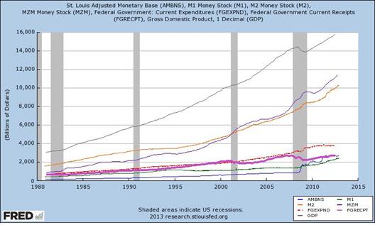
Figure 2: Six measures of MS and GDP. From top to bottom: GDP, MZM, M2, FGEXPND, FGRECPT, M1 and AMBNS. The general term EMS is plotted as Government Receipts (FGRECPT) and as Government Expenditures (FGEXPND) over the last 32 years.
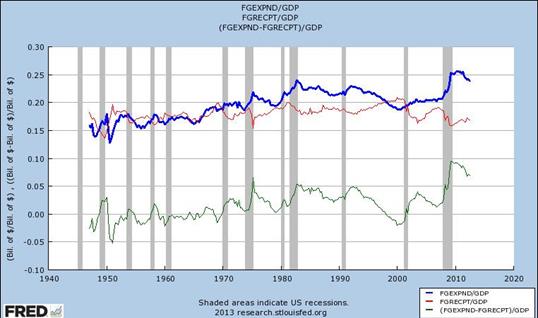
Figure 3: Three metrics of Government Nominal Tax Rate(NTR), Economic Tax Rate(ETR) and the Printed or Borrowed Rate(PBR) for last 66 years. ETR is the top dark line, NTR is the next line down and PBR is the bottom line.
Remaining Potential GDP Rate
When stimulus is used to accelerate an economy, Government Expenditures exceed Government Revenues. Part of the stimulus increases revenues the first year of application, and the remainder is available for future stimulation at the will of the savers. The future potential GDP is sum of PB/TR since the beginning of the currency.
Not developed here, the equation for the growth rate of Potential GDP (PGDPR) is
PGDPR = GDP*((Federal Expenses/Federal Receipts)-1).
The past 66 years of data in the United States results in the dramatic PGDPR graph shown in Figure 4.
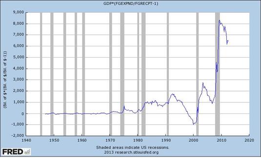
Figure 4: Sixty six years of data plotted to show the annual growth rate of Potential GDP. The rate has begun swinging wildly in the last few years.
Velocity of Money
Conventional Economics utilizes the concept of velocity of money to describe how efficiently a given money supply is used to reach a final GDP. The formula is
Velocity = GDP/Money Supply.
Utilizing Equation 4, substitute into the velocity equation by writing
Velocity = (G/(TR + PBR)) / Money Supply.
If we assume that G is the money supply as previously done in this paper, then we can write
Velocity = 1/ (NTR + PBR).
Now it can be seen that velocity is fundamentally related to the inverse of nominal tax rate plus the rate at which new money is added to the economy (when Government Expenditures is used as the money supply term). This neatly explains why velocity is so low under current United States Federal Reserve stimulus policies.
The Role of Banks
Citizens deposit their money (FRN) into banks with the result that banks record huge stocks of money on their books. All of this money can be traced from the yearly initial issue at some initial point in time. Banks make a practice of lending this money with the result that money stopped by saving is restarted on the GDP path. This is at risk to the bank because a promise is made to the depositor that the deposited money is available when in fact it has been loaned to another citizen! Amazingly, the loaned money returns to the bank under the name of another depositor as savings, allowing the bank to lend the money again! Strict bank rules limit the amount of debt-to-deposits created with this savings/return-to-the-GDP-path process. It is easy to see how the bank can profit from interest charged each borrower when the loans are made using money belonging to depositors!
It is also easy to see how banks can safely lend to Government when Government can replace the FRN as needed should a run on a bank occur!
The Valuation of Money
It is no surprise that money seems to have vastly different valuation depending upon who is holding money at any moment. As issuer who can print or deprint money, governments have a very generous attitude, thinking of money more as a tool than something to exchange for value. On the other hand, citizens vary from destitute who are desperate for money to rich folks who, not needing more money or work, value their time very highly indeed, thank you! Some citizens carefully shepherd their money and some look at money as a gift certificate to use as quickly as possible. The variety of perceptions and uses for money is without bound but it is obvious from Equation 1 that GDP is limited by tax rate and money supply. There is no bound for valuation, only for GDP.
Ultimately, the value of money can be logically be expected to depend upon availability. Logically, the more money Government prints, the less value per unit as with any commodity. Logically, the value of money should increase when Government deprints and go down when Government prints.
The role of savers in delaying continuation of the GDP stream should be re-emphasized. Much of the value of money depends upon the frugality of savers as well as the frugality with which Government prints, but the effects are very different in frame of time. Government prints by spending more than received with immediate effect. Savers spend in the future which may be tomorrow or years away. Future spending will be GDP = (remaining MS)/TR , an amount larger than immediate spending if TR is less than 0.5.
Backing Money With Value
The historical record of money contains a rich history of money issued as proxy for a commodity, usually a rare but durable material such as gold. Over time, backing has evolved in a direction favoring a fiat currency which means that the currency is only backed by the faith and credit of the issuing government. Citizens are willing to accept and hold fiat currency along with debt denominated in the currency so long as the currency is perceived as being difficult to acquire and having value when the decision is made to spend. Fear of value loss can be a very destabilizing factor as when citizens perceive a future rapid value change such as might follow a change in tax code or uncontrolled printing of new money.
Is Social Security Savings or Money Supply?
For a number of years, Social Security has collected more than was spent on retiree benefits with the reasoning that currently employed citizens should save for their retirement. How to invest many trillion dollars collected over many years was solved by investing with the Federal Government. Citizens assumed the role of the Federal Reserve!
Social Security has been a saving program for citizens but has become debt for government. Think about it! The Federal Treasury gives a bond to citizens (acting through the Social Security Trust Fund) and receives green Federal Reserve Notes (FRN) in return. The Federal Treasury gives a bond to the Federal Reserve and receives green Federal Reserve Notes (FRN) in return. The only difference between the Fed and citizens is that citizens earn their saved Federal Reserve Notes and the Fed simply prints their new Federal Reserve Notes.
That said, the difference between printing and earning is huge when considering how the transaction affects money supply. The act of delivering money to Government removes FRN from the outstanding money supply. Then Government gives citizens a bond and reissues FRN as a transfer to beneficiaries and spends the rest as a Federal Expenditure, thus reissuing FRN. The bond given citizens in this case is a promise to provide Social Security Benefits in the future to the extent defined by face value of the bonds.
Equation 1 can be used to follow the effects of this social experiment. To create this entitlement program, government raised taxes which has the effect of reducing the potential future GDP, and effectively lowers near term savings. Government then restored GDP by spending the tax revenue which increases the money supply. The social effect of helping the immediate beneficiaries of the tax and promising savers future replacement income created economic effects which shifted the economy into a Government defined model where Government owes Citizens trillions of future Dollars. Due to changing demographics, the Social Security Trust Fund is expected to be drawn down in future years. Government will have the choice of printing FRN or increased taxation to pay down the Treasury bonds owed by the Social Security Trust Fund.
How large is the Fiat Money Supply?
It is not difficult to estimate the size of the existing money supply with data available to the public when it is recognized that the money supply is held as both debt and FRN. Money held by the public (Private Investors) as Federal Government debt is tallied in the Federal Reserve data series FDHBPIN. Money initially issued to the Federal Treasury by the Federal Reserve and later issued to the public as FRN is tallied in data series FDHBFRBN. Money that has flowed through the Social Security System has resulted in debt to the government (data series FDHBATN) but no increase in the money supply. Money that has flowed into the hands of foreigners is tallied in data series FDHBFIN but is already counted in data series FDHBPIN so care must be exercised when using the FDHBFIN data. Figure 5 is a chart showing the two components of money supply as a ratio to GDP.
Money supply accounting can become confusing if an effort is made to follow Treasury operations. Assuming that all debt transactions are government debt, Federal Reserve-Treasury transactions create "double money", Treasury-citizen transactions are "single money", and Federal Reserve-citizen transactions cause no change in the debt-plus-FRN money supply. The "single money" situation occurs with FRN- debt exchanges between citizens and Federal Treasury where it is found that debt increases but FRN does not. Accounting confusion is avoided by leaving Total Government Debt out of the money supply calculation as was done in the paragraph above.
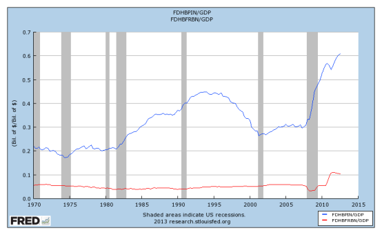
Figure 5: Total Money Supply on Two Lines. The top line is debt held by the public (Private Investors) and the bottom line is Federal Reserve Notes (FRN), both expressed as a ratio to GDP.
The money supply can also be estimated by adding all the Federal Deficits since the beginning of fiat money use. More exactly, this would be the grand sum of Federal Expenditures (FGEXPND) less Federal Receipts (FGRECPT), or the negative series Federal Savings (FGDEF). This method tracks well with the method above.
The apparent money supply coming from bank lending as calculated by the Federal Reserve can be found by subtracting the series FDHBFRBN and FDHBPIN from M2 or MZM. The remainder is estimated money supply contributed by deposit sourced lending.
Use the Simple Math to Formulate Governmental Policy
Money is a ubiquitous term. For purpose of discussing the role of money in policy, using the theory presented here, it is much better to use the term "token" when speaking of money as a means of exchange. Thus, don't say "A government worker receives money", say "A government worker receives a token". By using the term "token", the distinction that money is a transitory tool is emphasized.
Consider that armies, space programs and more complicated house building programs are all ways to put people to work at no long term cost to government because all cost are returned to government by taxes. On the other hand, pensions are a problem because they withdraw money from the GDP stream for long periods of time and are expected to grow. With pensions, the citizen cannot both have money and spend it unless the pension IS money and that is what has happened in the United States economy. Much of the invested pension money is held in the form of Treasury Bonds which are simply agreements with token holders to not spend their tokens now.
As a fundamental relationship, Equation 1 is useful to find balance between tax policy, GDP, and stimulus. From GDP = EMS/ETR, we easily see that increasing the Effective Money Supply (EMS) should increase GDP and increasing the Effective Tax Rate (ETR) should decrease GDP. Increasing EMS would result in the dilution of the existing money supply.
Excess expenditures, which are new money supply, survive the point-in-time GDP calculation as savings for the citizen and as debt on the Government balance sheet. Excess expenditures create a love/hate relationship with savers who love the savings but fear the additional competition from increased money supplies when the time comes to spend savings. We can use Equation 1 to determine the future GDP = PB/TR remaining as savings but we cannot predict when the future GDP will occur.
The effect of PBR in Equation 4 can be reduced by increasing the nominal tax rate (NTR). Money is no longer saved but may be spent immediately by Government. The depressing effect of increased tax rates may be mitigated with increased Government spending but expect a hidden effect of decreased saving.
While we have not discussed savings in depth, the dilution effect of increased money supply in Equation 4 can be reduced when Government borrows from Citizens rather than the Federal Reserve Bank. Citizens who choose to delay spending are accommodated by any Government borrowing of the Government's own evidence of debt. The practice was used heavily in WW2 when nearly all production was needed by Government for war production. Workers were encouraged to defer current spending with generous interest payments and pervasive savings campaigns. The practice was never abandoned but until recently was used to control spending by savers while continuing Government spending. During the recent past, Government has set interest rates to near zero, discouraging saving and encouraging savers to spend. The failure of savers to respond to the Government clues is worthy of further study.
Politics
Money plays an essential role in modern economies but fiat money must be created by governments run by decision makers. Money creation has short term effect and extended long term effect so the decision to print or deprint money becomes a dilemma and very political. Politics might be less rancorous if all decision makers had a common understanding of how money works.
What can be printed can be deprinted. Government can print at will but deprinting is done only by taxing which is much more difficult.
There is no need to mention the difficulty decision makers might find in deciding who should first receive the newly printed money.
Conclusion
Modern fiat money is a government creation that lives long after the initial introduction by government purchases. Once received by government beneficiaries, any newly created money is saved by recipients who return the money into the economy at an unknown future time. New fiat money survives until government runs a budget surplus which will effectively remove fiat paper from the money supply.
The only thing more valuable than money is the trade that money buys.
Copyright 2013 by Roger Sparks
Revised 3/22/2013
Comments are invited. Please contact rsparks@elltel.net
Note: The original "Money Begins" was withdrawn 3/20/2013 and re-written to de-emphasize the formula GDP = MS/(TR +PBR). Hopefully, this new version is easier to read and understand. RCS
A PDF version is avaliable at Fiat Money Begins.